4 Results
4.1 cEOF spatial patterns
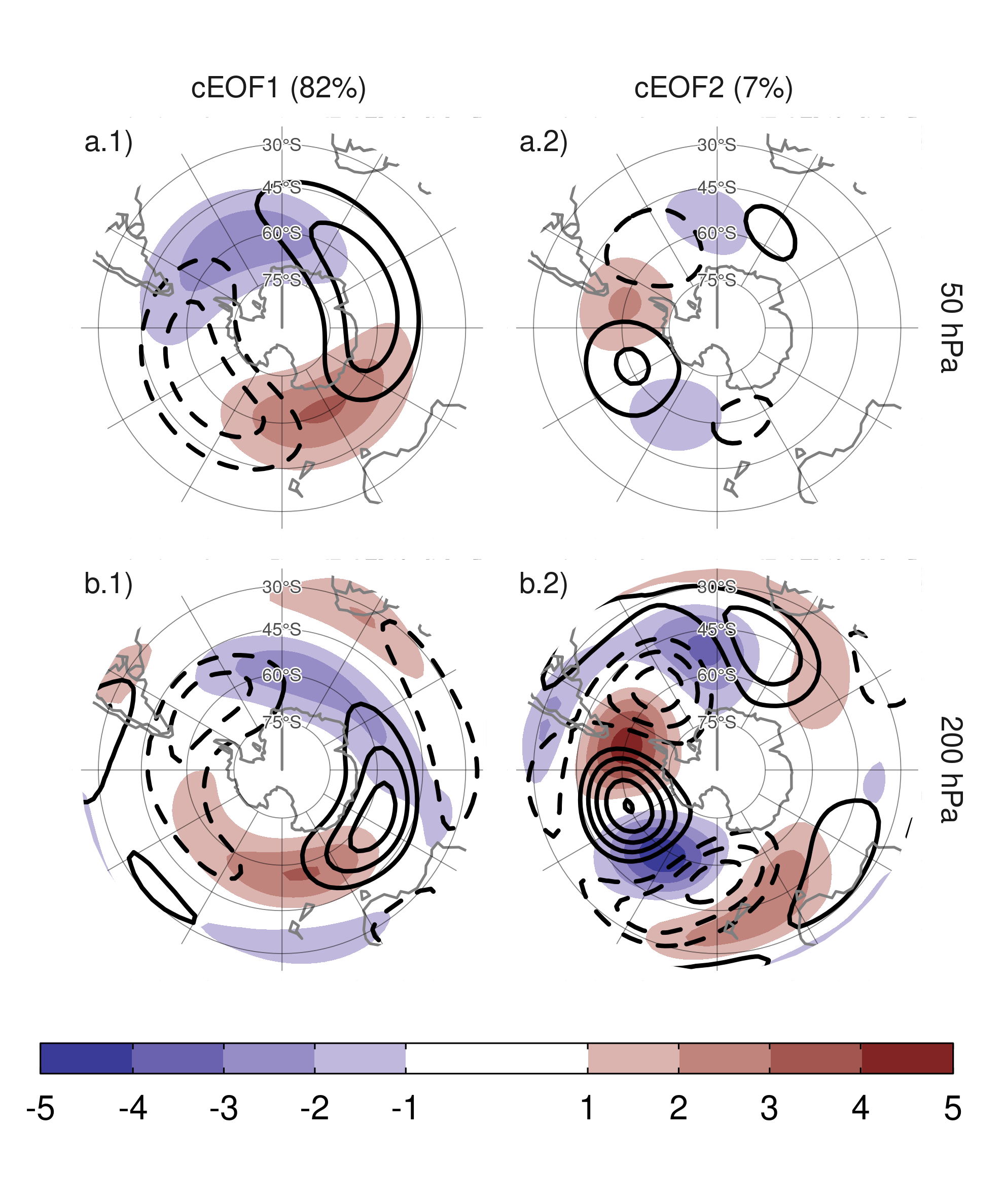
Figure 2: Spatial patterns for the two leading cEOFs of SON geopotential height zonal anomalies at 50 hPa and 200 hPa for the 1979 – 2019 period. The shading (contours) corresponds to 0º (90º) phase. Arbitrary units. The proportion of variance explained for each mode with respect to the zonal mean is indicated in parenthesis.
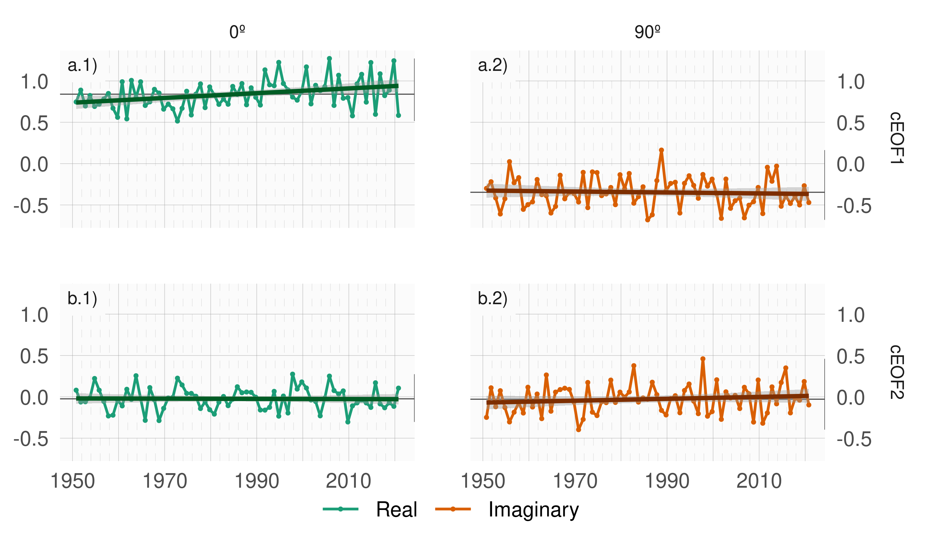
Figure 3: Time series of the two leading cEOFs of SON geopotential height zonal anomalies at 50 hPa and 200 hPa. cEOF1 (row a) and cEOF2 (row b) separated in their 0º (column 1) and 90º (column 2) phase. Dark straight line is the linear trend. Black horizontal and vertical line mark the mean value and range of each time series, respectively.
To describe the variability of the circulation zonal anomalies, the spatial and temporal parts of the first two leading cEOFs of zonal anomalies of geopotential height at 50 hPa and 200 hPa, computed jointly at both levels, are shown in Figures 2 and 3. The first mode (cEOF1) explains 82% of the variance of the zonally anomalous fields, while the second mode (cEOF2) explains a smaller fraction (7%). In the spatial patterns (Fig. 2), the 0º and the 90º phases are in quadrature by construction, so that each cEOF describe a single wave-like pattern whose amplitude and position (i.e. phase) is controlled by the magnitude and phase of the temporal cEOF. The wave patterns described by these cEOFs match the patterns seen in the standard EOFs of Figure 1.
The cEOF1 (Fig. 2 column 1) is a hemispheric wave 1 pattern with maximum amplitude at high latitudes. At 50 hPa the 0º cEOF1 has the maximum of the wave 1 at 150ºE and at 200 hPa, the maximum is located at around 175ºE indicating a westward shift with height. The cEOF2 (Fig. 1 column 2) shows also a zonal wave-like structure with maximum amplitude at high latitudes, but with shorter spatial scales. In particular, the dominant structure at both levels is a wave 3 but with larger amplitude in the pacific sector. There is no apparent phase shift with height but the amplitude of the pattern is greatly reduced in the stratosphere, which is consistent with the the fact that the cEOF2 computed separately for 200 hPa explains a bit more variance than the cEOF2 computed separately for 50 hPa (11% vs. 3%, respectively). This suggest that this barotropic mode represents mainly tropospheric variability.
There is no significant simultaneous correlation between cEOFs time series. Both cEOFs show year-to-year variability but show no evidence of decadal variability (Fig. 3). The 0º cEOF has a non-zero temporal mean which, as discussed in Section 3.3, is due to the fact that the temporal mean of zonal anomalies need to be captured by the cEOFs. The other indices have almost zero temporal mean, which indicates that only cEOF1 includes variability that significantly projects onto the mean zonal anomalies. This is consistent with the fact that the mean zonal anomalies of geopotential height are very similar to the cEOF1 (\(r^2\) = 98%) and not similar to the cEOF2 (\(r^2\) = 0%).
A significant positive trend in the 0º phase of cEOF1 is evident (Fig. 3a.1, p-value = 0.0037) while there is no significant trend in any of the phases of cEOF2. The positive trend in the 0º cEOF1 translates into a positive trend in cEOF1 magnitude, but not systematic change in phase (not shown). This long-term change indicates an increase in the magnitude of the high latitude zonal wave 1.
4.2 cEOFs Regression maps
4.2.1 Geopotential
In the previous section, cEOF analysis was applied to zonal anomalies derived by removing the zonally mean values in order to isolate the main characteristics of the main zonal waves characterizing the circulation in the SH. In this section we compute regression fields using the full fields of the variables in order to describe the influence of the cEOFs on the temporal anomalies.
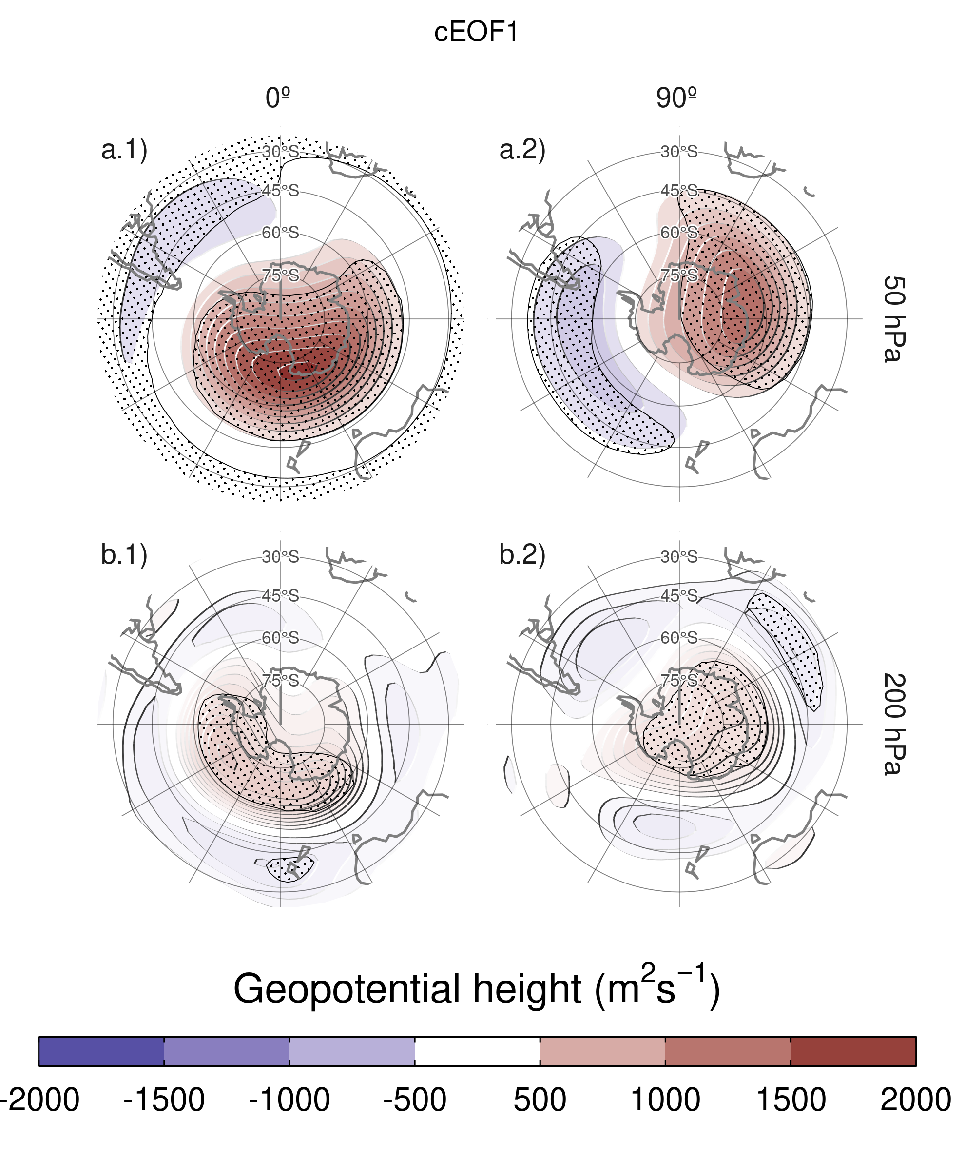
Figure 4: Regression of SON geopotential height anomalies (\(m^2s^{-1}\)) with the (column 1) 0º and (column 2) 90º phases of the first cEOF for the 1979 – 2019 period at (row a) 50 hPa and (row b) 200 hPa. These coefficients come from multiple linear regression involving the 0º and 90º phases. Areas marked with dots have p-values smaller than 0.01 adjusted for False Detection Rate.
Figure 4 shows regression maps of SON geopotential height anomalies upon cEOF1. At 50 hPa (Figure 4 row a), the 0º cEOF1 is associated with a positive centre located over the Ross Sea. The correlation between the 0º cEOF1 and the zonal mean zonal wind at 60ºS and 10hPa is -0.59 (CI: -0.76 – -0.35), indicating a moderate relationship with the SON stratospheric jet. The 90º cEOF1 is associated with a distinctive wave 1 pattern with maximum over the coast of East Antarctica. At 200 hPa (Figure 4 row b) the 0º cEOF1 shows a single centre of positive anomalies spanning West Antarctica surrounded by opposite anomalies in lower latitudes, with its centre shifted slightly eastward compared with the upper-level anomalies. The 90º cEOF1 shows a much more zonally symmetrical pattern resembling the negative SAM phase (e.g. Fogt and Marshall 2020). Therefore, the magnitude and phase of the cEOF1 are associated with the magnitude and phase of a zonal wave mainly in the stratosphere.
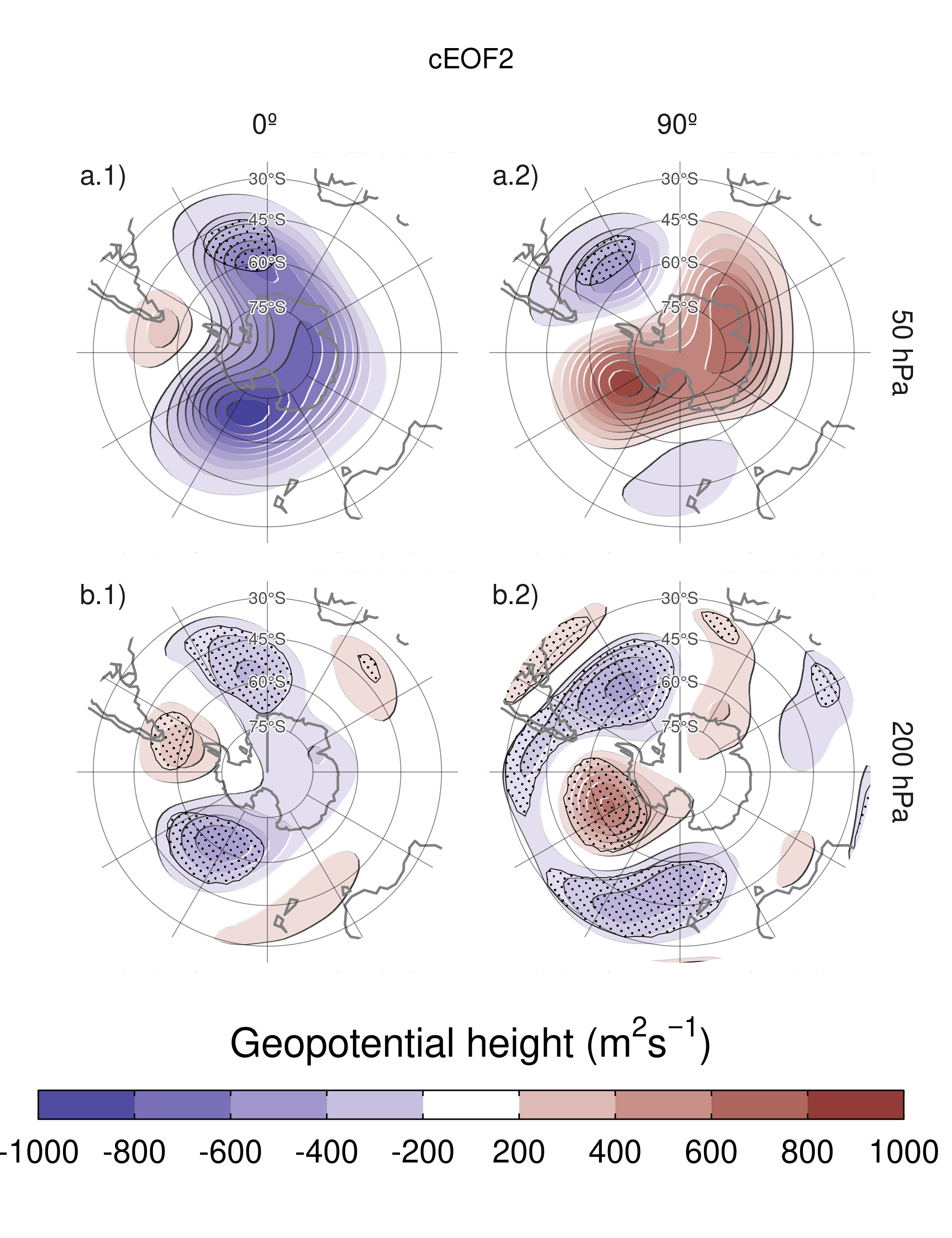
Figure 5: Same as Figure 4 but for cEOF2.
Figure 5 shows the regression maps of geopotential height anomalies upon the cEOF2. In the troposphere (Fig. 5 row a) the regression maps show wave trains similar to those identified for cEOF2 patterns (Fig 2). Regressed anomalies associated with the 0º cEOF2 are 1/4 wavelength out of phase with those associated with the 90º cEOF2. All fields have a dominant zonal wave 3 limited to the western hemisphere, over the Pacific and Atlantic Oceans. cEOF2 then represents an equivalent barotropic wave train that is very similar to the the PSA Patterns (Mo and Paegle 2001). Comparing the location of the positive anomaly near 90ºW in column 2 of Figure 5 with Figures 1.a and b from Mo and Paegle (2001), the 0º cEOF2 regression map could be identified with PSA2, while the 90º cEOF2 resembles PSA1.
These wave patterns are also present in the stratosphere (Fig. 5 row a) supporting their equivalent barotropic nature. But also present is a monopole over the pole with negative sign associated with the 0º cEOF2 and positive sign associated with the 90º cEOF2. This monopole might indicate strengthening of the polar vortex associated with positive values of the 0º cEOF2 and weakening associated with negative values of 0º cEOF2. However, since these anomalies are not statistically significant, this feature should not be overinterpreted.
4.2.2 Temperature and Ozone
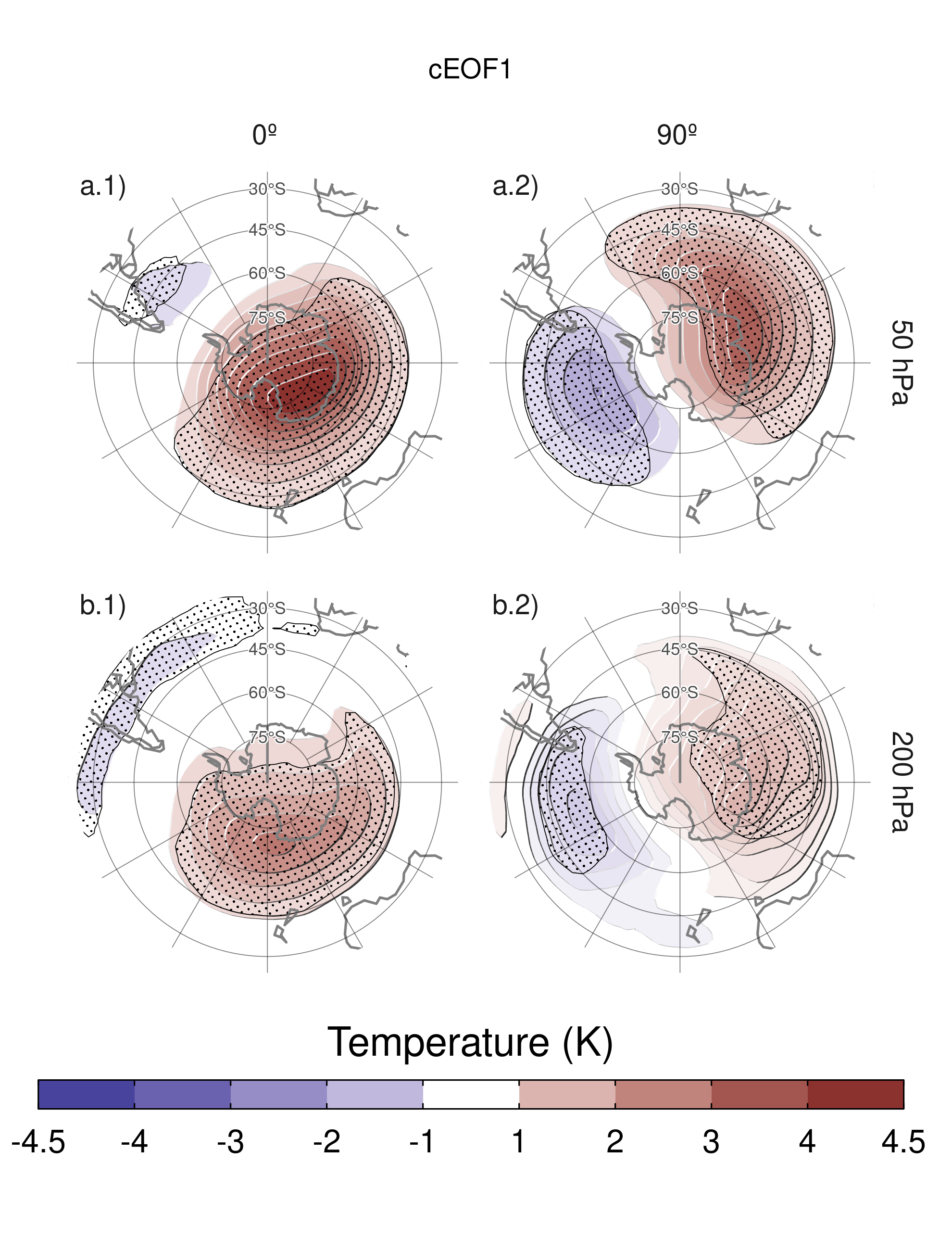
Figure 6: Same as Figure 4 but for air temperature (K).
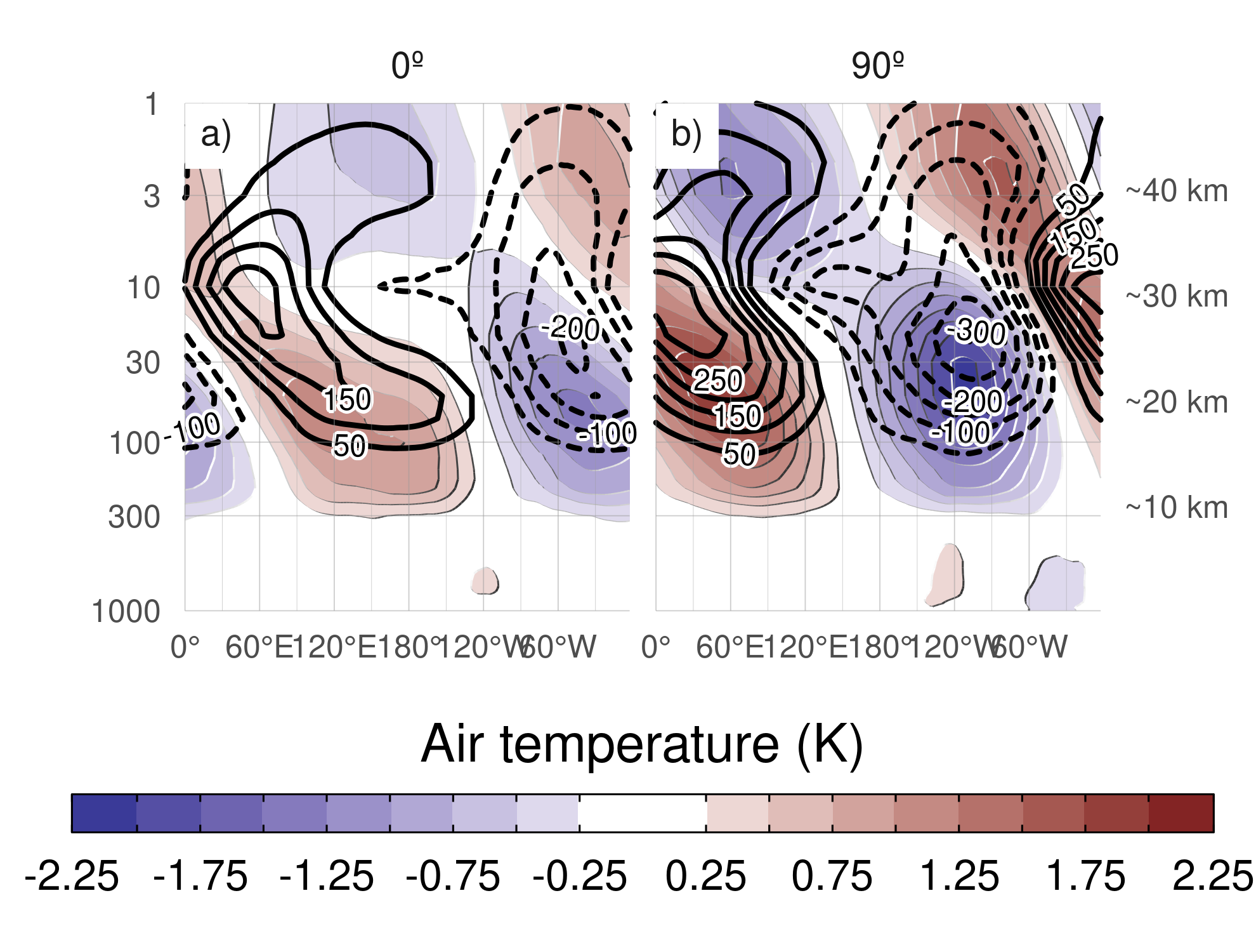
Figure 7: Regression of SON zonal anomalies averaged between 75°S and 45°S of mean air temperature (shaded, Kelvin) and ozone mixing ratio (contours, negative contours with dashed lines, labels in parts per billion by mass) with the (a) 0º and (b) 90º phase of the cEOF1 for the 1979 – 2019 period.
The signature of cEOFs variability on air temperature was also evaluated. Figure 6 shows regression maps of air temperature anomalies at 50 hPa and 200 hPa upon cEOF1. The distribution of temperature regression coefficients at 50 hPa and at 200 hPa mirror the geopotential height regression maps at 50 hPa (Fig. 4). In both levels, the 0º cEOF1 is associated with a positive centre over the South Pole with its centre moved slightly towards 150ºE (Fig. 6 column 1). On the other hand, the regression maps on the 90º cEOF1 show a clearer wave 1 pattern with its maximum around 60ºE.
Figure 7 shows the vertical distribution of the regression coefficients on cEOF1 from zonal anomalies of air temperature and of ozone mixing ratio averaged between 75°S and 45°S. Temperature zonal anomalies associated with cEOF1 show a clear wave 1 pattern for both 0º and 90º phases throughout the atmosphere above 250 hPa with a sign reversal above 10 hPa. As a result of the hydrostatic balance, this is the level in which the geopotential anomaly have maximum amplitude (not shown).
The maximum ozone regressed anomalies coincide with the minimum temperature anomalies above 10 hPa and with the maximum temperature anomalies below 10 hPa (Fig. 7). Therefore, the ozone zonal wave 1 is negatively correlated with the temperature zonal wave 1 in the upper stratosphere, and positively correlated in the upper stratosphere. This change in phase is observed in ozone anomalies forced by planetary waves that reach the stratosphere. In the photochemically-dominated upper stratosphere, cold temperatures inhibit the destruction of ozone, explaining the opposite behaviour for both variables as were elucidated with dynamical chemical models (Hartmann and Garcia 1979; Wirth 1993; Smith 1995). On the other hand, in the advectively-dominated lower stratosphere, ozone anomalies are 1/4 wavelength out of phase with horizontal and vertical transport, which are in addition 1/4 wavelength out of phase with temperature anomalies, resulting in same sign anomalies for the response of both variables (Hartmann and Garcia 1979; Wirth 1993; Smith 1995).
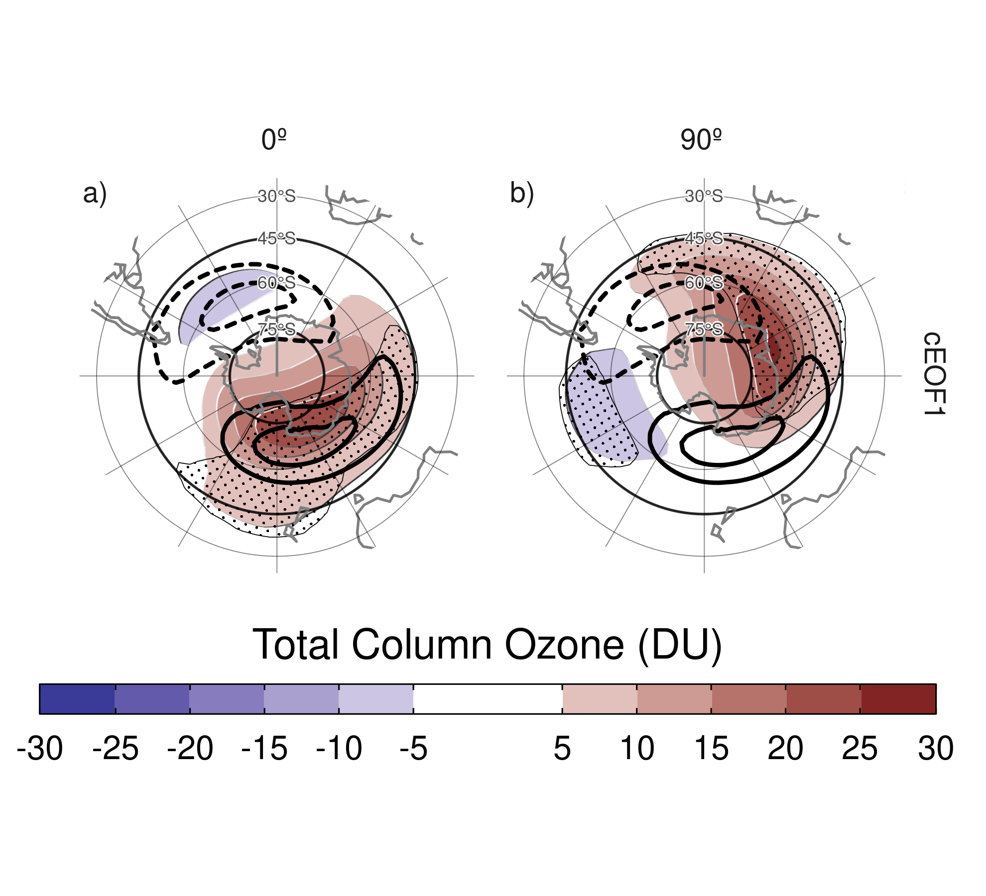
Figure 8: Regression of SON mean Total Column Ozone anomalies (shaded, Dobson Units) with the (a) 0º and (b) 90º phases of the cEOF1 for the 1979 – 2019 period. On contours, the mean zonal anomaly of Total Column Ozone (negative contours in dashed lines, Dobson Units). Areas marked with dots have p-values smaller than 0.01 adjusted for False Detection Rate.
The regression maps of TCO anomalies upon cEOF1 (Fig. 8) show zonal wave 1 patterns associated with both components of cEOF1. The climatological position of the springtime Ozone minimum (ozone hole) is outside the South Pole and towards the Weddell Sea (e.g. Grytsai 2011). Thus, the 0º cEOF1 regression field (Figure 8a) coincides with the climatological position of the ozone hole, while it is 90° out of phase for the 90º cEOF1. The temporal correlation between the amplitudes of TCO planetary wave 1 and the amplitude of cEOF1 is 0.79 (CI: 0.63 – 0.88), while the correlation between their phases is -0.85 (CI: -0.92 – -0.74). Consequently, cEOF1 is strongly related with the SH ozone variability.
4.3 PSA
| PC | Real | Imaginary |
|---|---|---|
| PSA1 | 0.26 (CI: -0.04 – 0.52) | 0.82 (CI: 0.69 – 0.9) |
| PSA2 | 0.79 (CI: 0.63 – 0.88) | -0.02 (CI: -0.32 – 0.29) |
Given the similarity between the cEOF2 related-associated structures (Fig. 5) and documented PSA patterns, we study the relationship between them. Table 2 shows the correlations between the two PSA indices and the time series for 0º and 90º phases of cEOF2. As visually anticipated by Figure 5, there is a large positive correlation between PSA1 and 90º cEOF2, and between PSA2 and 0º cEOF2. On the other hand, there is no significant relationship between PSA1 and 0º cEOF2, and between PSA2 and 90º cEOF2. As a result, cEOF2 represents well both the spatial structure and temporal evolution of the PSA modes, so it is possible to make an association between its two phases and the two PSA modes. That is, the phase election for cEOF2 that maximises the relationship between ENSO and 90º cEOF2, also maximises the association between cEOF2 components and PSA modes (not shown).
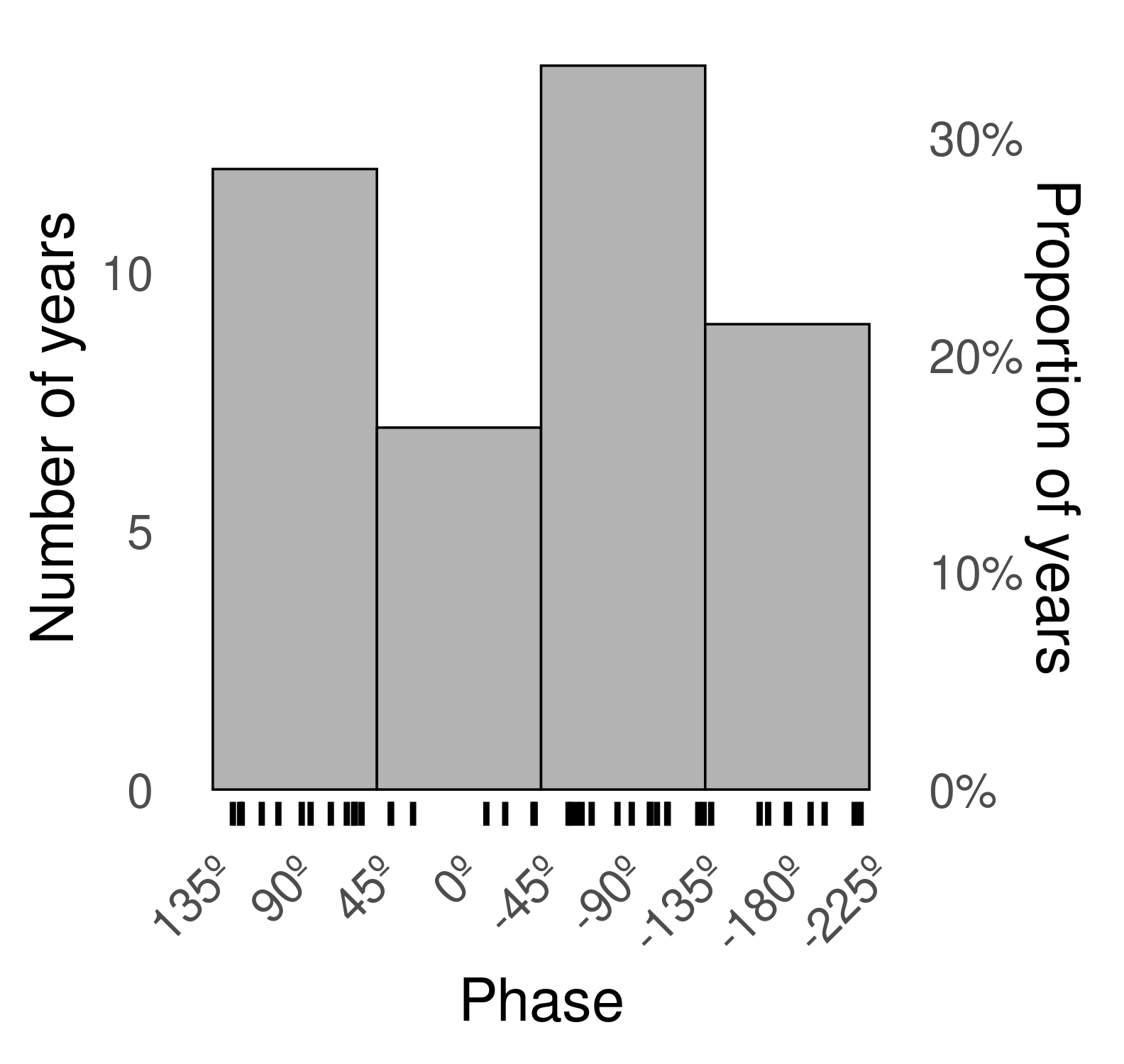
Figure 9: Histogram of phase distribution of cEOF2 phase for the 1979 – 2019 period. Bins are centred at 90º, 0º, -90º, -180º with a binwidth of 90º. The small vertical lines near the horizontal axis mark the observations.
Figure 9 shows an histogram that counts the number of SON seasons in which the cEOF2 phase was close to each of the four particular phases (positive/negative of 0º and 90º phases), with the observations for each season marked as rugs on the horizontal axis. In 62% of seasons cEOF2 has a phase similar to either the negative or positive 90º phase, making the 90º phase the most common phase. This is also the phase that is most correlated with ENSO by the definition of the 0° phase as described in Section 3.
Therefore, by virtue of being the most common phase, the 90º cEOF2 explains more variance than the 0º cEOF2. Conventional EOF analysis will therefore tend to separate them relatively cleanly, with the EOF representing the 90º cEOF2 always leading the one representing the 0º cEOF2. This phase preference is in agreement with Irving and Simmonds (2016), who found a bimodal distribution to PSA-like variability (compare our Figure 9 with their Figure 6).
4.4 SAM
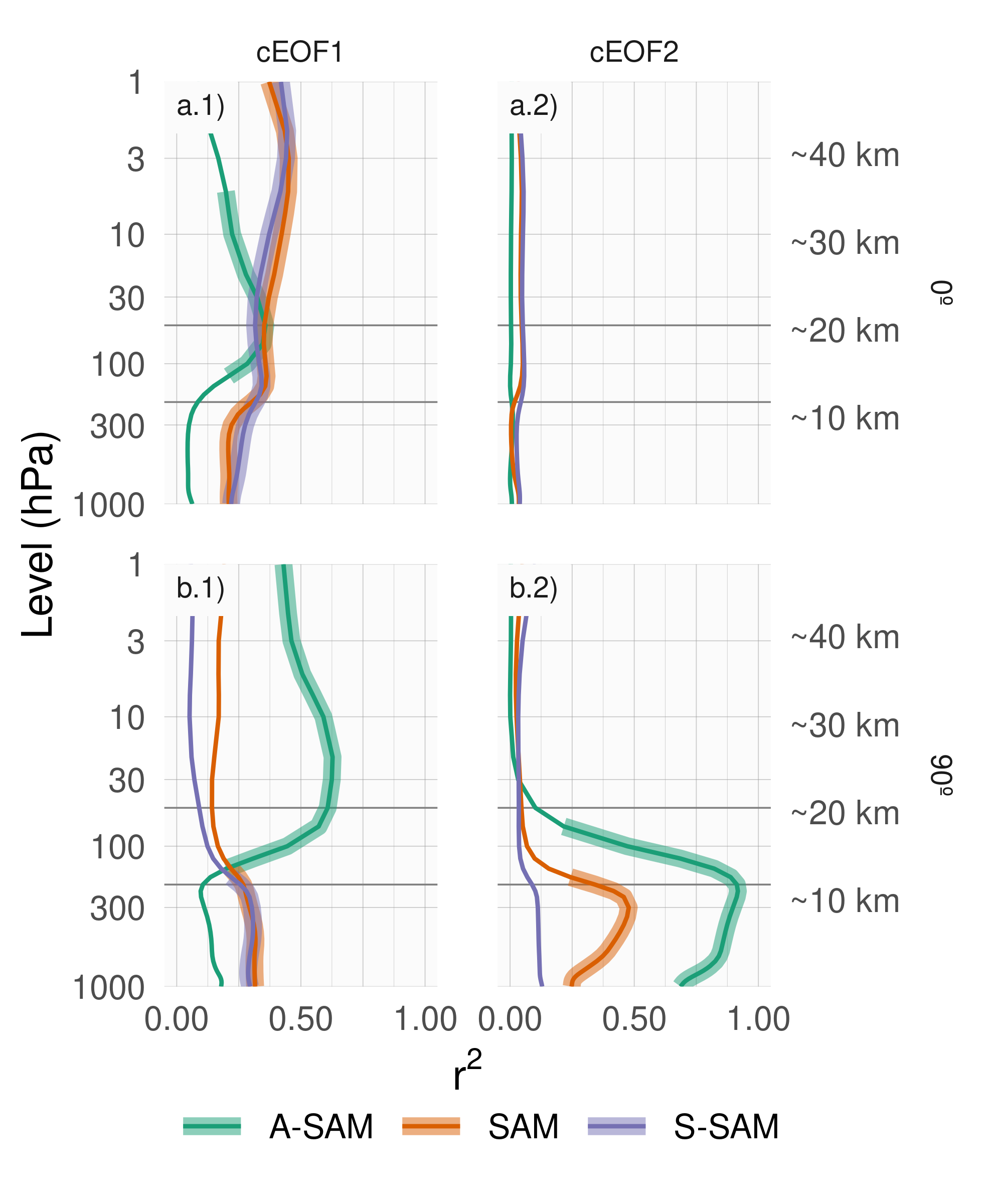
Figure 10: Coefficient of determination (\(r^2\)) between each component of cEOFs and the SAM, Asymmetric SAM (A-SAM) and Symmetric SAM (S-SAM) indices computed at each level for the 1979 – 2019 period. Thick lines represent estimates with p-value < 0.01 corrected for False Detection Rate (Benjamini and Hochberg 1995).
We now explore the relationship between SAM and the cEOFs motivated by the resemblance between cEOFs regression maps and SAM patterns shown in Section 4.2. We computed the coefficient of determination between the cEOFs time series and the three SAM indices (SAM, A-SAM and S-SAM) defined by Campitelli, Díaz, and Vera (2022a) at each vertical level (Fig. 10). The SAM index is statistically significantly correlated with the 0º cEOF1 in all levels, and with the 90º cEOF1 and 90º cEOF2 in the troposphere. On the other hand, correlations between SAM and the 0º cEOF2 are non-significant.
The relationship between the SAM and cEOF1 in the troposphere is explained entirely by the zonally symmetric component of the SAM as shown by the high correlation with the S-SAM below 100 hPa and the low and statistically non-significant correlations between the A-SAM and either the 0º or 90º cEOF1. In the stratosphere, the 0º cEOF1 is correlated with both A-SAM and S-SAM, while the 90º cEOF1 is highly correlated only with the A-SAM. These correlations are consistent with the regression maps of geopotential height in Figure 4 and their comparison with those obtained for SAM, A-SAM and S-SAM by Campitelli, Díaz, and Vera (2022a).
In the case of 90º cEOF2, its correlation with the SAM for the troposphere is associated with the asymmetric variability of the SAM. Indeed, the 90º cEOF2 shares up to 92% variance with the A-SAM and only 12% at most with the S-SAM (Figure 10.b2). Such extremely high correlation between A-SAM and 90º cEOF2 suggests that the modes obtained in this work are able to characterise the zonally asymmetric component of the SAM described previously by Campitelli, Díaz, and Vera (2022a).
4.5 Tropical sources of cEOFs variabitliy

Figure 11: Regression of SST (K, left column) and streamfunction zonal anomalies (\(m^2/s\times10^-7\), shaded) with their corresponding activity wave flux (vectors) (right column) upon cEOF2 different phases (illustrated in the lower-left arrow) for the 1979 – 2019 period. Areas marked with dots have p-values smaller than 0.01 adjusted for FDR.
The connections between cEOFs and tropical sources of variability were also assessed. Figure 11 shows the regression maps of Sea Surface Temperature (SST) and streamfunction anomalies at 200 hPa upon standardised cEOF2. As well as regression maps for the 0º and 90º phases, we include corresponding regressions for two intermediate directions (corresponding to 45° and 135°).
The 90º cEOF2 (second row) is associated with strong positive SST anomalies on the Central to Eastern Pacific and negative anomalies over an area across northern Australia, New Zealand the South Pacific Convergence Zone (SPCZ) (Figure 11.b1). The regression field of SST anomalies bears a strong resemblance with canonically positive ENSO (Bamston, Chelliah, and Goldenberg 1997). Indeed, there is a significant and very high correlation (0.76 (CI: 0.6 – 0.87)) between the ONI and the 90º cEOF2 time series. In addition to the Pacific ENSO-like pattern, there are also positive anomalies in the western Indian Ocean and negative values in the eastern Indian Ocean, resembling a positive IOD (Saji et al. 1999). Consistently, the correlation between the 90º cEOF2 and the DMI is 0.62 (CI: 0.38 – 0.78).
The 90º cEOF2 is associated with strong wave-like streamfunction anomalies emanating from the tropics (Figure 11.b2), both from the Central Pacific sector and the Indian Ocean. The atmospheric response associated with 90º cEOF2 is then consistent with the combined effect of ENSO and the IOD on the extratropics: with SST anomalies inducing anomalous tropical convection that in turn excite Rossby waves propagating meridionally towards higher latitudes (Mo 2000; Cai et al. 2011a; Nuncio and Yuan 2015).
However, the cEOF2 is not associated with the same tropical SST anomaly patterns at all their phases Figure 11.d1 and d2 show that the 0º cEOF2 is not associated either with any significant SST nor streamfunction anomalies in the tropics. As a result, the correlation between the 0º cEOF2 and ENSO is not significant (0 (CI: -0.3 – 0.3)). Meanwhile, Rows a and c in Fig. 11 show that the intermediate phases are still associated with significant SST regressed anomalies over the Pacific Ocean, but at slightly different locations. The 135º phase is associated with SST anomalies in the central Pacific (Fig. 11a.1), while the 45º phase is associated with SST anomalies in the eastern Pacific, which correspond roughly to the Central Pacific and Eastern Pacific “flavours” of ENSO, respectively (Fig. 11c.1) (Kao and Yu 2009). Both phases are also associated with wave trains generated in the region surrounding Australia and propagates toward the extra-tropics, although less intense than the ones associated with the 90º phase.
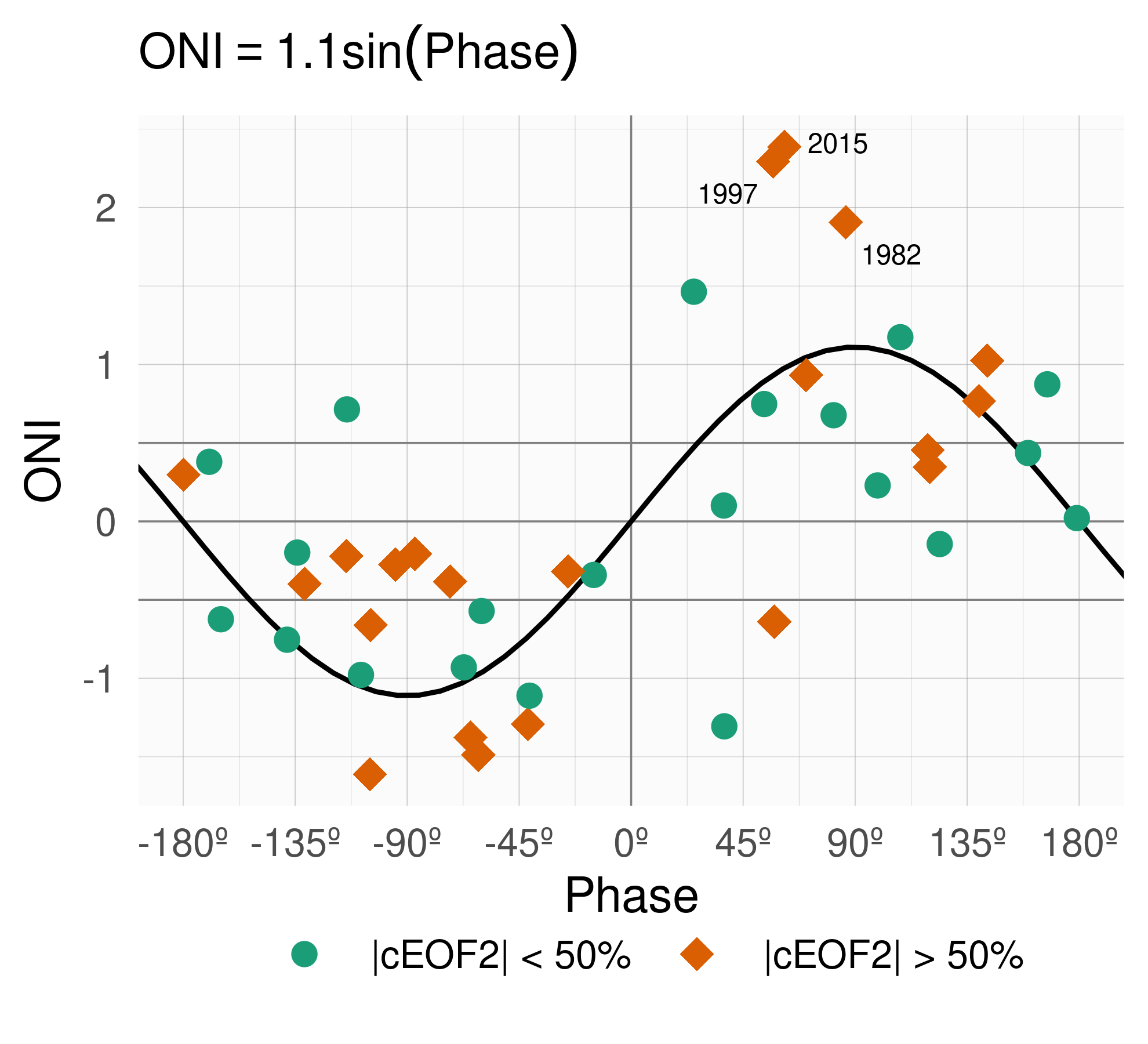
Figure 12: SON ONI values plotted against cEOF2 phase for the 1979 – 2019 period. Years with magnitude of cEOF2 greater (smaller) than the 50th percentile are shown as orange diamonds (green circles). Black line is the fit ONI ~ sin(phase) computed by weighted OLS using the magnitude of the cEOF2 as weights.
To further explore the relationship between tropical forcing and phases of the cEOF2, Figure 12 shows the ONI plotted against the cEOF2 phase for each SON trimester between 1979 and 2019, highlighting years in which the magnitude of cEOF2 is above the median. In years with positive (negative) ONI, the cEOF2 phase is mostly around 90º (-90°). In the neutral ENSO seasons, the cEOF2 phase is much more variable. The black line in Figure 12 is a sinusoidal fit of the relationship between ONI and cEOF2 phase. The \(r^2\) corresponding to the fit is 0.57, statistically significant with p-value < 0.001, indicating a quasi-sinusoidal relation between these two variables.
The correlation between the absolute magnitude of the ONI and the cEOF2 amplitude is 0.45 (CI: 0.17 – 0.66). However, this relationship is mostly driven by the three years with strongest ENSO events in the period (2015, 1997, and 1982) which coincide with the three years with strongest cEOF2 magnitude (not shown). If those years are removed, the correlation becomes non-significant (0.04 (CI: -0.28 – 0.35)). Furthermore, even when using all years, the Spearman correlation –which is robust to outliers– is also non-significant (0.2, p-value = 0.21). Therefore, although the location of tropical SST anomalies seem to have an effect in defining the phase of the cEOF2, the relationship between the magnitude of cEOF2 and ONI remains uncertain and might be only evident in very strong ENSO events, that are scarce in the historical observational record.
We conclude that the wave train represented by cEOF2 can be both part of the internal variability of the extratropical atmosphere and forced by tropical SSTs. In the former case, the wave train has little phase preference. However, when cEOF2 is excited by tropical SST variability, it tends to remain locked to the 90º phase. This explains the relative over-abundance of years with cEOF2 near positive and negative 90º phase in Figure 9.
Unlike the cEOF2 case, there are no significant SST regressed anomalies associated with either the 0º or 90º cEOF1 (Sup. Figure 15). Consistently, streamfunction anomalies do not show any tropical influence. Instead, the 0º and 90º cEOF1 are associated with zonally propagating wave activity fluxes in the extra-tropics around 60ºS, except for an equatorward flow from the coast of Antarctica around 150ºE in the 0º phase. This suggests that the variability of cEOF1 is driven primary by the internal variability of the extra-tropics.
4.6 cEOFs surface impacts
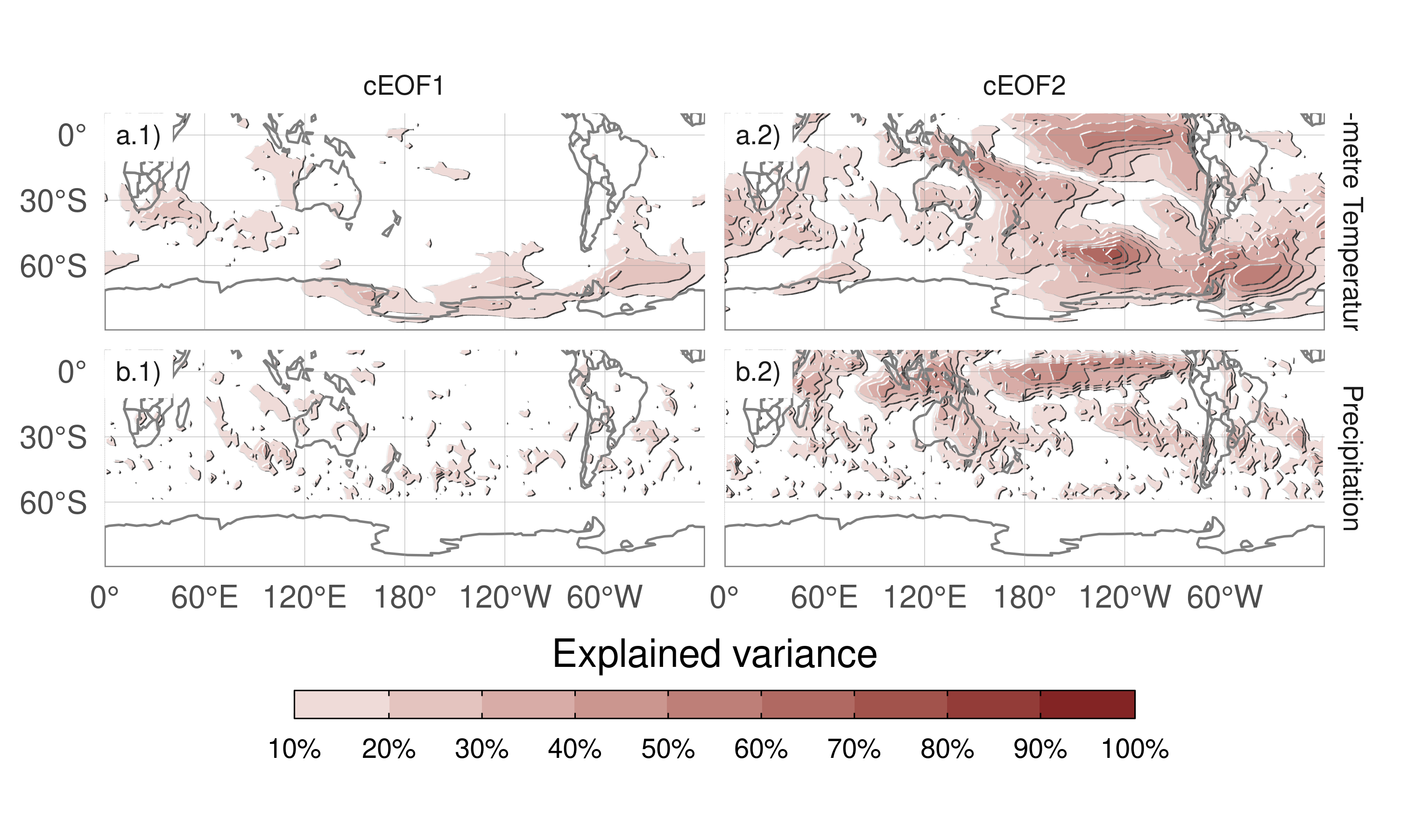
Figure 13: Explained variance (\(r^2\) as percentage) of 2-metre temperature (row a) and precipitation (row b) anomalies by the regression upon cEOF1 (column 1) and cEOF2 (column 2).
The influence of cEOFs variability in the anomalies of both 2-metre air temperature and precipitation in the SH was also explored. Figure 13 shows the 2-meter temperature and precipitation anomalies explained variance by the multiple linear model of both 0º and 90º cEOF1 (column 1), and both 0º and 90º cEOF2 (column 2). The variance explained by cEOF1 for precipitation anomalies and temperature anomalies in most regions is extremely low, except for the northern tip of the Antarctic Peninsula, northern Weddell Sea and the Ross Sea coast (Fig. 13a.1).
This lack of strong relationship between the cEOF1 and SST, temperature and precipitation might be surprising considering the correlation between the cEOF1 and the SAM (Fig. 10 column 1) and the correlation between SAM and Central Pacific SST, temperature east and west of the Antarctic Peninsula, and with precipitation in western Australia (Fogt and Marshall 2020). There are two main reasons for this. First, the correlation between cEOF1 and the SAM in the troposphere is modest, with less than 50% of shared variance (Fig. 10 column 1), so these indices are not expected to be equivalent to each other. Second, Campitelli, Díaz, and Vera (2022a) showed that the strong relationship between the SAM and Pacific SSTs and temperature anomalies around the Antarctic Peninsula is mainly due to the asymmetric part of the SAM. Meanwhile, the cEOF1 is significantly correlated only with the symmetric part of the SAM (Fig. 10 column 1), which by itself is not significantly correlated with surface temperatures in that area.
On the other hand, the cEOF2 explained variance is greater than 50% in some regions for both variables (Fig. 13 column 2). For 2-metre temperature, there are high values in the tropical Pacific and the SPCZ, as well as the region following an arc between New Zealand and the South Atlantic, with higher values in the Southern Ocean. Over the continents, there are moderate values of about 30% variance explained in southern Australia, Southern South America and the Antarctic Peninsula. For precipitation, there are high values over the tropics. At higher latitudes, moderate values are observed over eastern Australia and some regions of southern South America.
Since the cEOF1 has a relatively weak signal in the surface variables explored here, we will only focus on the cEOF2 influence. Figure 14 shows regression maps of 2-metre temperature (column 1) and precipitation (column 2) anomalies upon different phases of standardised cEOF2.
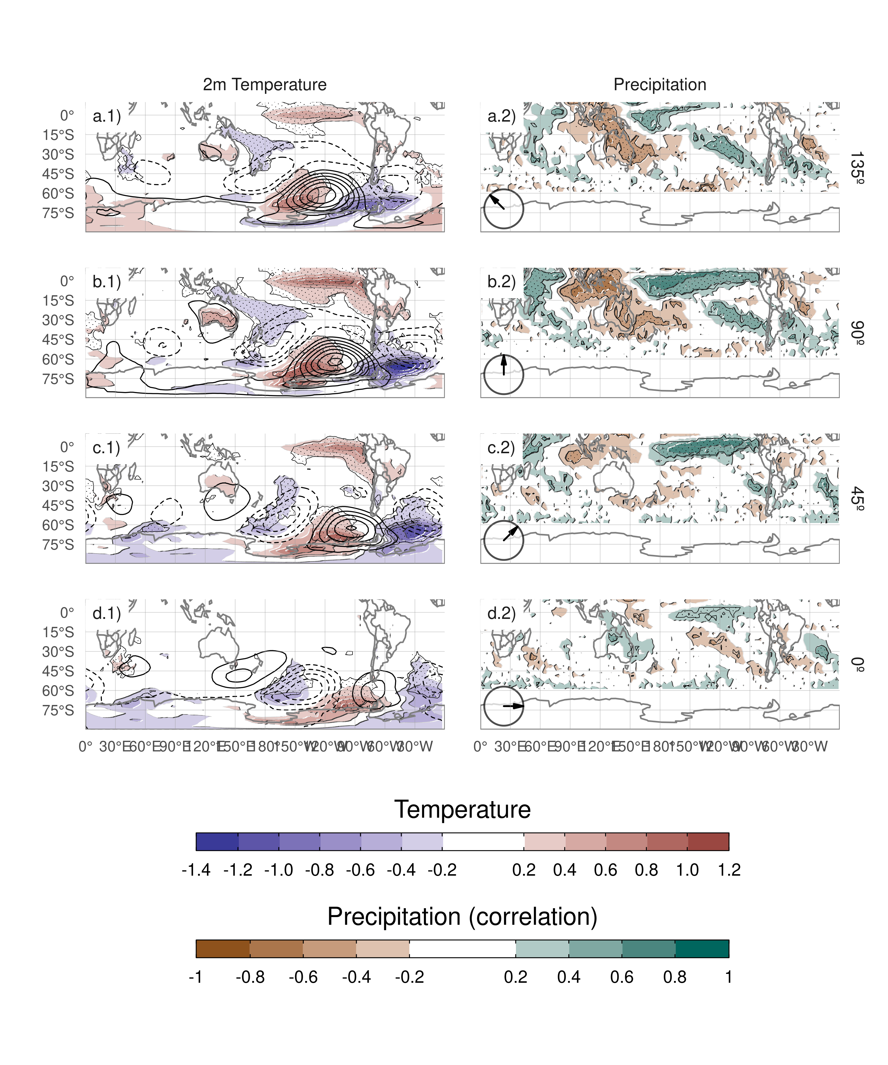
Figure 14: Regression of SON mean 2-meter temperature (K, shaded) and 850 hPa geopotential height (m, contours) (column 1), and precipitation (correlation, column 2) upon different phases of cEOF2. For the 1979 – 2019. Areas marked with dots have p-values smaller than 0.01 adjusted for False Detection Rate.
Temperature anomalies associated with the 90º cEOF (Fig. 14.b1) show positive values in the tropical Pacific, consistent with SSTs anomalies associated with the same phase (Fig. 11.b1). At higher latitudes there is a wave-like pattern of positive and negative values that coincide with the nodes of the 850 hPa geopotential height regression patterns. This is consistent with temperature anomalies produced by meridional advection of temperature by the meridional winds arising from geostrophic balance. Over the continents, the 90º cEOF2 (Fig. 14b.1) is associated with positive regressed temperature anomalies in southern Australia and negative regressed anomalies in southern South America and the Antarctic Peninsula, that are a result of the wave train described before.
The temperatures anomalies associated with the 0º cEOF2 (Fig. 14d.1) are less extensive and restricted to mid and high latitudes.
Over the continents, the temperature anomalies regressions are non significant, except for positive anomalies near the Antarctic Peninsula.
Tropical precipitation anomalies associated with the 90º cEOF2 are strong, with positive anomalies in the central Pacific and western Indian, and negative anomalies in the eastern Pacific (Fig. 14b.2). This field is consistent with the SST regression map (Fig. 14b.1) as the positive SST anomalies enhance tropical convection and the negative SST anomalies inhibits it.
In the extra-tropics, the positive 90º cEOF2 is related to drier conditions over eastern Australia and the surrounding ocean, that it is similar signal as the one associated with ENSO (Cai et al. 2011a). However, the 90º cEOF2 is not the phase most correlated with precipitation in that area. The 135º phase (an intermediate between positive 90º and 180º cEOF2) component is associated with stronger and more extensive temporal correlations with precipitation over Australia and New Zealand, consistent with the effect of ENSO on precipitation in that region. These anomalies are probably related to the direct effect of vertical anomalies of the Southern Oscillation and less so to the large-scale circulation anomalies described by cEOF2 (Cai et al. 2011b). Circulation anomalies associated with the Indian Ocean Dipole could also play a role (Cai et al. 2011b).
Over South America, the 90º cEOF2 has positive correlations with precipitation in South Eastern South America (SESA) and central Chile, and negative correlations in eastern Brazil. This correlation field matches the springtime precipitation signature of ENSO (e.g. Cai et al. 2020) and it is also similar to the precipitation anomalies associated with the A-SAM (Campitelli, Díaz, and Vera 2022a). This result is not surprising considering the close relationship of the 90º cEOF2 with both ONI and A-SAM index, which was shown previously. Furthermore, it consolidates the identification of the cEOF2 with the PSA pattern. Resembling the relationship between ONI and the phase of cEOF2 (Fig. 12), there is a cEOF2 phase dependence of the precipitation anomalies in SESA (not shown).
The correlation coefficients between precipitation anomalies and the 0º cEOF2 (Fig. 14d.2) are weaker than for 90º cEOF2. There is a residual positive correlation in the equatorial eastern Pacific and small, not statistically significant positive correlations over eastern Australia and negative ones over New Zealand.