3 Data and Methods
3.1 Data
We used monthly geopotential height, air temperature, ozone mixing ratio, and total column ozone (TCO) at 2.5º longitude by 2.5º latitude of horizontal resolution and 37 vertical isobaric levels from the European Centre for Medium-Range Weather Forecasts Reanalysis version 5 [ERA; Hersbach et al. (2019)] for the period 1979 – 2019. Most of our analysis is restricted to the post-satellite era to avoid confounding factors arising from the incorporation of satellite observations, but we also used the preliminary back extension of ERA5 from 1950 to 1978 (Bell et al. 2020) to describe long-term trends. We derived streamfunction at 200 hPa from ERA5 vorticity using the FORTRAN subroutine FISHPACK (Adams, Swartztrauber, and Sweet 1999) and we computed horizontal wave activity fluxes following Plumb (1985). Sea Surface Temperature (SST) monthly fields are from Extended Reconstructed Sea Surface Temperature (ERSST) v5 (Huang et al. 2017) and precipitation monthly data from the CPC Merged Analysis of Precipitation (CMAP, P. Xie and Arkin 1997), with a 2º and 2.5º horizontal resolution, respectively. The rainfall gridded dataset is based on information from different sources such as rain gauge observations, satellite inferred estimations and the NCEP-NCAR reanalysis, and it is available from 1979 to the present.
The Oceanic Niño Index (ONI, Bamston, Chelliah, and Goldenberg 1997) comes from NOAA’s Climate Prediction Center and the Dipole Mode Index (DMI, Saji and Yamagata 2003) from Global Climate Observing System Working Group on Surface Pressure.
3.2 Methods
The study is restricted to the spring season, defined as the September-October-November (SON) trimester. We compute seasonal means for the different variables, averaging monthly values weighted by the number of days in each month. We use the 200 hPa level to represent the upper troposphere and 50 hPa to represent the lower stratosphere.
We computed the amplitude and phase of the TCO wave 1 by averaging (area-weighted) the data of each SON between 75°S and 45°S, and then extracting the wave-1 component of the Fourier spectrum. We chose this latitude band because it is wide enough to capture most of the relevant anomalies of SH mid-latitudes.
We computed the level-dependent SAM index as the leading EOF of year-round monthly geopotential height anomalies south of 20ºS at each level for the whole period (Baldwin and Thompson 2009). We further split the SAM into its zonally symmetric and zonally asymmetric components (S-SAM and A-SAM indices respectively) following Campitelli, Díaz, and Vera (2022a). The method consists in first computing the leading EOF of monthly geopotential height anomalies at each level and then computing the zonal mean and the zonal anomalies from its spatial pattern. We then project each level’s monthly geopotential height fields onto the corresponding EOF field, the zonally symmetric field and the zonally asymmetric fields to obtain time series corresponding to the full SAM, the symmetric SAM and the asymmetric SAM, respectively.
Seasonal indices of the PSA patterns (PSA1 and PSA2) were calculated, in agreement with Mo and Paegle (2001), as the third and fourth EOFs of seasonal mean anomalies for 500-hPa geopotential heights at SH.
Linear trends were computed by Ordinary Least Squares (OLS) and the 95% confidence interval was computed assuming a t-distribution with the appropriate residual degrees of freedom (D. Wilks 2011).
3.3 Complex Empirical Orthogonal Functions (cEOF)
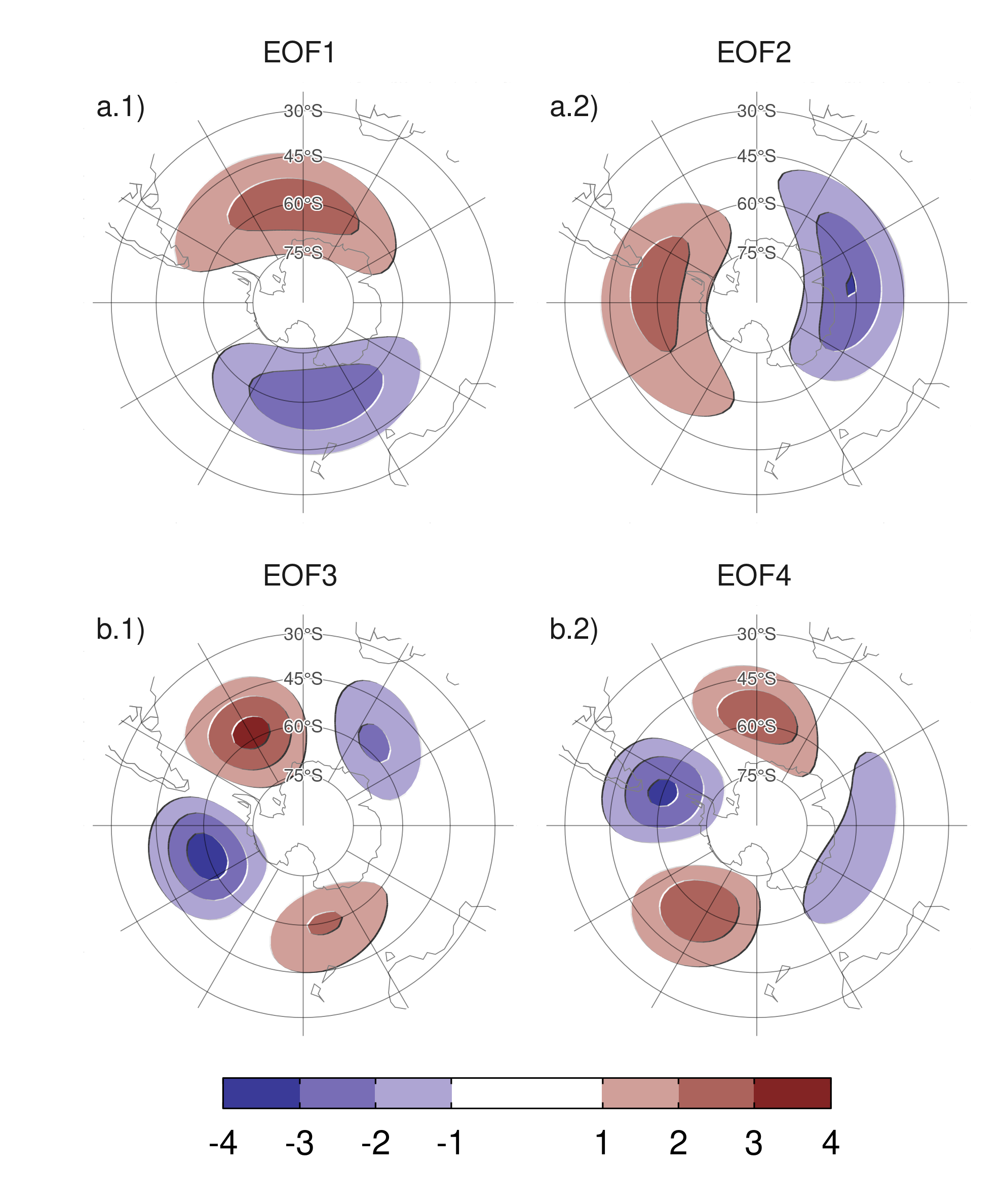
Figure 1: Spatial patterns of the four leading EOFs of SON geopotential height zonal anomalies at 50 hPa south of 20º S for the 1979 – 2019 period (arbitrary units).
In the standard EOF analysis, zonal waves may appear as pairs of (possibly degenerate) EOFs representing similar patterns but shifted in phase (Horel 1984). Figure 1 shows the four leading EOFs of SON geopotential height zonal anomalies at 50 hPa south of 20º S. It is clear that the first two EOFs represent a single phase-varying zonal wave 1 pattern and the last two represent a similarly phase-varying pattern with higher wavenumber and three centres of action shifted by 1/4 wavelength (90º in frequency space).
To describe the phase-varying nature of these two wave patterns, one way is to combine each pair of EOFs into indices of amplitude and phase. So, for instance, the amplitude of the wave 1-like EOF could be measured as \(\sqrt{\mathrm{PC1}^2 + \mathrm{PC2}^2}\) and its phase as \(\tan^{-1} \left ( \frac{\mathrm{PC2}}{\mathrm{PC1}} \right )\) (where \(\mathrm{PC1}\) and \(\mathrm{PC2}\) are the time series associated with each EOF). However, this rests on visual inspection of the spatial patterns and only works properly if both phases appear clearly in different EOFs, which is not guaranteed by construction. In particular, this does not work with the wave 1 pattern depicted as the leading EOF in 200 hPa geopotential height zonal anomalies (not shown).
On the other hand, a better alternative for describing phase-varying waves is to use Complex Empirical Orthogonal Functions (cEOF) analysis (Horel 1984). Each cEOF is a set of complex-valued spatial patterns and time series. The real and imaginary components of the complex spatial pattern can be thought of as representing two spatial patterns that are shifted by 1/4 wavelength by construction, similar to EOF1 and EOF2 in Figure 1. In this paper we use the term 0º cEOF and 90º cEOF to refer to each part of the whole cEOF. The actual field reconstructed by each cEOF is then the linear combination of the two spatial fields weighted by its respective time series. This is analogous to how any sine wave can be constructed by the sum of a sine wave and cosine wave with different amplitude but constant phase. This means that cEOFs naturally represent phase-varying wave-like patterns that change location as well as amplitude.
For instance, when the phase of the wave matches the 0º phase, then the 0º phase time series is positive, and the 90º phase time series is zero. Similarly, when the phase of the wave matches the 90º phase, the 90º phase time series is positive, and the 0º phase time series is zero. The intermediate phases have non-zero values in both time series.
In traditional EOFs, the resulting modes are not unique, and instead are defined up to sign, which corresponds to a rotation in the complex plane of either 0 or \(\pi\). In the same way, cEOFs are defined up to a rotation in the complex plane of any value between 0 and \(2\pi\) (Horel 1984).
cEOFs are computed in the same way as traditional EOFs except that the data is first augmented by computing its analytic signal. This is a complex number whose real part is the original series and whose imaginary part is the original data shifted by 90º at each spectral frequency – i.e. its Hilbert transform. The Hilbert transform is usually understood in terms of time-varying signal. However, in this work we apply the Hilbert transform at each latitude circle, level, and at each SON mean (i.e. the signal only depends on longitude). Since each latitude circle is a periodic domain, this procedure does not suffer from edge effects.
We first applied cEOF analysis to geopotential height zonal anomalies south of 20ºS at 50 and at 200 hPa. Figure 2 a.1 shows the spatial patterns of the two leading cEOF. The 0º phase is plotted with shaded contours and the 90º phase, with black contours. The two phases of the leading cEOF are very similar to the two leading EOFs shown in Figure 1 and represent a zonal wave 1 pattern; the 0º phase is roughly the EOF1 and the 90º phase is roughly the EOF2).
| 200 hPa | cEOF1 | cEOF2 | cEOF3 |
|---|---|---|---|
| cEOF1 | 0.29 | 0.01 | 0.03 |
| cEOF2 | 0.00 | 0.59 | 0.02 |
| cEOF3 | 0.00 | 0.00 | 0.01 |
Table 1 shows the coefficient of determination between time series of the amplitude of each cEOF across levels. There is a high degree of correlation between the magnitude of the respective cEOF1 and cEOF2 at each level. The spatial patterns of the 50 hPa and 200 hPa cEOFs are also similar (not shown).
Both the spatial pattern similarity and the high temporal correlation of cEOFs computed at 50 hPa and 200 hPa suggest that these are, to a large extent, modes of joint variability. This motivates the decision of performing cEOF jointly between levels. Therefore cEOFs were computed using data from both levels at the same time. In that sense each cEOF has a spatial component that depends on longitude, latitude and level, and a temporal component that depends only on time.
Because we are computing the cEOFs of zonal anomalies and not temporal anomalies, the cEOFs need to account for the time-mean zonal anomalies. These will tend to be represented by the leading cEOF, which therefore will have a non-zero temporal mean.
As mentioned before, the choice of phases is arbitrary and equally valid. But to make the interpretation easier, we chose the phase of each cEOF so that either the 0º cEOF or the 90º cEOF is aligned with meaningful variables in our analysis. This procedure does not create spurious correlations, it only takes an existing relationship and aligns it with a specific phase.
Preliminary analysis showed that the first cEOF was closely related to the zonal wave 1 of TCO and the second cEOF was closely related to ENSO. Therefore, we chose the phase of cEOF1 so that the time series corresponding to the 0º cEOF1 has the maximum correlation with the zonal wave 1 of TCO between 75°S and 45°S. Similarly, we chose the phase of cEOF2 so that the coefficient of determination between the ONI and the 0º cEOF2 is minimised, which also nearly maximises the correlation with the 90º cEOF2.
In Section 4.6 we show regressions of precipitation and temperature associated with intermediate phases. For those plots, we rotated the cEOFs by 1/4 wavelength by multiplying the complex time series by \(\cos(\pi/4) + i\sin(\pi/4)\) and computing the regression on those rotated timeseries.
While we compute these complex principal components using data from 1979 to 2019, we extended the complex time series back to the 1950 – 1978 period by projecting monthly geopotential height zonal anomalies standardised by level south of 20ºS onto the corresponding spatial patterns.
We performed linear regressions to quantify the association between the cEOFs and other variables (e.g. geopotential height, temperature, precipitation, and others). For each cEOF, we computed regression maps by fitting a multiple linear model involving both the 0º and the 90º phases. To obtain the linear coefficients of a variable \(X\) with the 0º and 90º phase of each cEOF we fit the equation
\[ X(\lambda, \phi, t) = \alpha(\lambda, \phi) \operatorname{cEOF_{0^\circ}} + \beta(\lambda, \phi) \operatorname{cEOF_{90^\circ}} + X_0(\lambda, \phi) + \epsilon(\lambda, \phi, t) \]
where \(\lambda\) and \(\phi\) are the longitude and latitude, \(t\) is the time, \(\alpha\) and \(\beta\) are the linear regression coefficients for 0º and 90º phases respectively, \(X_0\) and \(\epsilon\) are the constant and error terms respectively.
We evaluated statistical significance using a two-sided t-test and, in the case of regression maps, p-values were adjusted by controlling for the False Discovery Rate (Benjamini and Hochberg 1995; D. S. Wilks 2016) to avoid misleading results from the high number of regressions (Walker 1914; Katz and Brown 1991).
3.4 Computation procedures
We performed all analysis in this paper using the R programming language (R Core Team 2020), using data.table (Dowle and Srinivasan 2020) and metR (Campitelli 2020) packages. All graphics are made using ggplot2 (Wickham 2009). We downloaded data from reanalysis using the ecmwfr package (Hufkens 2020) and indices of ENSO and Indian Ocean Dipole (IOD) with the rsoi package (Albers and Campitelli 2020). The paper was rendered using knitr and rmarkdown (Y. Xie 2015; Allaire et al. 2020).