Wraping around ggplot2
Elio Campitelli
2023-10-30
Source:vignettes/wraping-around-ggplot2.Rmd
wraping-around-ggplot2.Rmdggperiodic is a simple package that tries to make plotting periodic data easier. The core idea is that you can specify the period that your data represents and then, at plotting, time, you define the range that it should be wrapped around. To see it in action, let’s first create some periodic data with period between 0° and 360°:
x <- seq(0, 360 - 10, by = 10)*pi/180
y <- seq(-90, 90, by = 10)*pi/180

Z <- expand.grid(x = x, y = y)
Z$z <- with(Z, 1.2*sin(x)*0.4*sin(y*2) -
               0.5*cos(2*x)*0.5*sin(3*y) +
               0.2*sin(4*x)*0.45*cos(2*x))
Z$x <- Z$x*180/pi
Z$y <- Z$y*180/pi
Since the vale of z at x = 0 and at
x = 360 is the same, having both would be redundant and
also create bias when computing statistics because the same point would
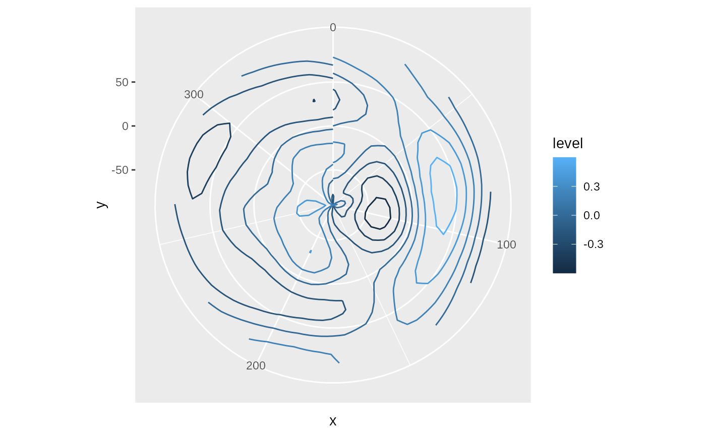
be double counted. But when plotting, there’s a problem
library(ggplot2)
ggplot(Z) +
  geom_contour(aes(x, y, z = z, color = ..level..)) +
  coord_polar()
#> Warning: The dot-dot notation (`..level..`) was deprecated in ggplot2 3.4.0.
#> ℹ Please use `after_stat(level)` instead.
#> This warning is displayed once every 8 hours.
#> Call `lifecycle::last_lifecycle_warnings()` to see where this warning was
#> generated.
With ggperiodic you can explicitly specify the period that your data represents and then wrap it around any arbitrary range. By printing, you can see the period of each of the periodic variables.
library(ggperiodic)
#>
#> Attaching package: 'ggperiodic'
#> The following object is masked from 'package:stats':
#>
#>     filter
Z <- periodic(Z, x = c(0, 360))
head(Z)
#>    x   y           z
#> 1  0 -90 -0.25000000
#> 2 10 -90 -0.18056111
#> 3 20 -90 -0.12361453
#> 4 30 -90 -0.08602886
#> 5 40 -90 -0.03806684
#> 6 50 -90  0.04875725
#> x = [0; 360]
To manually wrap the data around a range, you can use the same syntax:
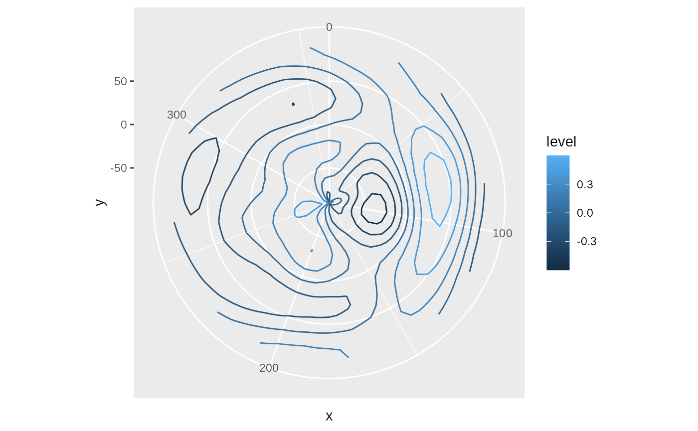
This can be done manually, but ggplot2 will do it automatically, by default wrapping the data around the period.
ggplot(Z) +
  geom_contour(aes(x, y, z = z, color = ..level..)) +
  coord_polar()
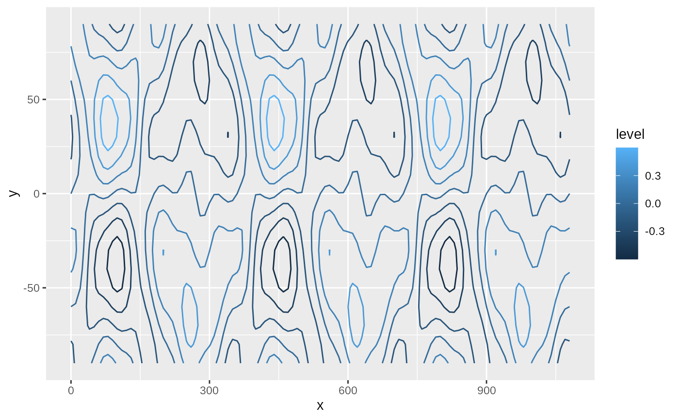
But it’s easy to change the wrapping range using the same syntax. For example, if we want to see three copies of the data
ggplot(Z, x = c(0, 360)*3) +
  geom_contour(aes(x, y, z = z, color = ..level..))