Computes a linear regression with stats::.lm.fit and returns the estimate and, optionally, standard error for each regressor.
Usage
FitLm(y, ..., intercept = TRUE, weights = NULL, se = FALSE, r2 = se)

ResidLm(y, ..., intercept = TRUE, weights = NULL)

Detrend(y, time = seq_along(y))
Arguments
- y
numeric vector of observations to model
- ...
numeric vectors of variables used in the modelling
- intercept
logical indicating whether to automatically add the intercept
- weights
numerical vector of weights (which doesn't need to be normalised)
- se
logical indicating whether to compute the standard error
- r2
logical indicating whether to compute r squared
- time
time vector to use for detrending. Only necessary in the case of irregularly sampled timeseries
Value
FitLm returns a list with elements
- term
the name of the regressor
- estimate
estimate of the regression
- std.error
standard error
- df
degrees of freedom
- r.squared
Percent of variance explained by the model (repeated in each term)
- adj.r.squared
r.squared` adjusted based on the degrees of freedom)
ResidLm returns a numeric vector of the same length as y.
It represents the residuals (anomalies) of the linear model.
The result is centered at approximately 0 (the trend is removed, and the mean is subtracted–Derived from the calculation of the least squares method).
Detrend returns a numeric vector of the same length as y.
It represents the detrended data with the original mean preserved.
Mathematically, it is residuals + mean(y).
If there's no complete cases in the regression, NAs are returned with no
warning.
Details
The functions provide different ways to handle linear trends:
ResidLm: Use this to compute anomalies. It subtracts the linear trend (including the intercept), effectively removing both the long-term trend and the mean. This corresponds to the standard "detrending and anomaly" step in climate analysis.
Detrend: Use this to remove the slope (trend) while retaining the physical magnitude of the data. It subtracts the linear trend but adds the original mean back. Ideally suited for visualizing data without the distraction of long-term trends while keeping the values in their original level.
Examples
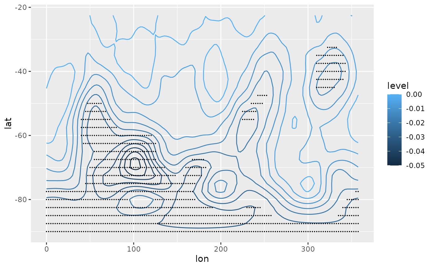
# Linear trend with "signficant" areas shaded with points
library(data.table)
library(ggplot2)
system.time({
  regr <- geopotential[, FitLm(gh, date, se = TRUE), by = .(lon, lat)]
})
#>    user  system elapsed
#>   0.201   0.000   0.201

ggplot(regr[term != "(Intercept)"], aes(lon, lat)) +
    geom_contour(aes(z = estimate, color = after_stat(level))) +
    stat_subset(aes(subset = abs(estimate) > 2*std.error), size = 0.05)


# Using stats::lm() is much slower and with no names.
if (FALSE) { # \dontrun{
system.time({
  regr <- geopotential[, coef(lm(gh ~ date))[2], by = .(lon, lat)]
})
} # }
# Using stats::lm() is much slower and with no names.
if (FALSE) { # \dontrun{
system.time({
regr <- geopotential[, coef(lm(gh ~ date))[2], by = .(lon, lat)]
})
} # }