
How to make a generic stat in ggplot2
En español: Como hacer un stat genérico en ggplot2For a while now I’ve been thinking that, yes, ggplot2 is awesome and offers a lot of geoms and stats, but it would be great if it could be extended with new user-generated geoms and stats. Then I learnt that ggplot2 actually has a pretty great extension system so I could create my own geoms I needed for my work or just for fun. But still, creating a geom from scratch is an involved process that doesn’t lend itself to simple transformations.
Finally, I thought of a possible solution: create a generic stat –a tabula rasa, if you will– that can work on the data with any function. Natively ggplot2 offers stat_summary(), but it’s only meant to be used with, well, summary statistics. What I wanted was something completely generic and this is my first try.
Below is the code for stat_rasa() (better name pending). It works just like any other stat except that it works with any function that takes a data.frame and returns a transformed data.frame that can be interpreted by the chosen geom.
# ggproto object
StatRasa <- ggplot2::ggproto("StatRasa", ggplot2::Stat,
  compute_group = function(data, scales, fun, fun.args) {
     # Change default arguments of the function to the
     # values in fun.args
     args <- formals(fun)
     for (i in seq_along(fun.args)) {
        if (names(fun.args[i]) %in% names(fun.args)) {
           args[[names(fun.args[i])]] <- fun.args[[i]]
        }
     }
     formals(fun) <- args

     # Apply function to data
     fun(data)
})

# stat function used in ggplot
stat_rasa <- function(mapping = NULL, data = NULL,
                      geom = "point",
                      position = "identity",
                      fun = NULL,
                      ...,
                      show.legend = NA,
                      inherit.aes = TRUE) {
   # Check arguments
   if (!is.function(fun)) stop("fun must be a function")

   # Pass dotted arguments to a list
   fun.args <- match.call(expand.dots = FALSE)$`...`

   ggplot2::layer(
      data = data,
      mapping = mapping,
      stat = StatRasa,
      geom = geom,
      position = position,
      show.legend = show.legend,
      inherit.aes = inherit.aes,
      check.aes = FALSE,
      check.param = FALSE,
      params = list(
         fun = fun,
         fun.args = fun.args,
         na.rm = FALSE,
         ...
      )
   )
}
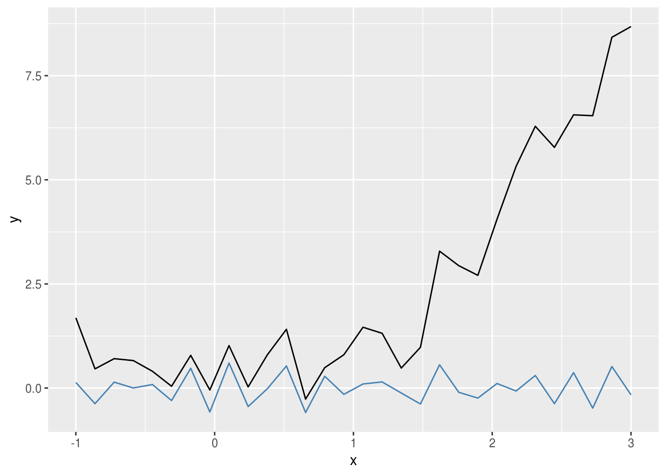
For example, let’s say we want to quickly glance at detrended data. We then create a very simple function
Detrend <- function(data, method = "lm", span = 0.2) {
   if (method == "lm") {
      data$y <- resid(lm(y ~ x, data = data))
   } else {
      data$y <- resid(loess(y ~ x, span = span, data = data))
   }
   as.data.frame(data)
}
and pass it to stat_rasa()
library(ggplot2)
set.seed(42)
x <- seq(-1, 3, length.out = 30)
y <- x^2 + rnorm(30)*0.5
df <- data.frame(x = x, y = y)
ggplot(df, aes(x, y)) +
   geom_line() +
   stat_rasa(geom = "line", fun = Detrend, method = "smooth",
             color = "steelblue")
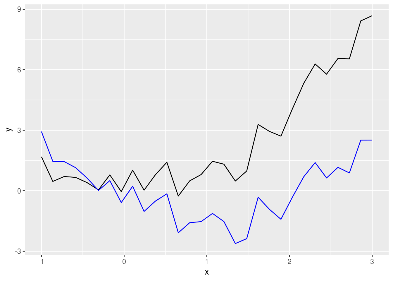
We can get better legibility and less typing by creating a wrapper function with a more descriptive name.
stat_detrend <- function(...) {
   stat_rasa(fun = Detrend, ...)
}

ggplot(df, aes(x, y)) +
   geom_line() +
   stat_detrend(method = "lm", color = "blue", geom = "line")
Another case could be calculating contours from an irregular grid. Since ggplot2::stat_contour() uses grDevices::contourLines(), it needs values defined in a regular grid, but there’s a package called contoureR that can compute contours from irregularly spaced observations. With stat_rasa() we can integrate it with ggplot2 effortlessly by creating a small function and using geom = "path".
IrregularContour <- function(data, breaks = scales::fullseq,
                             binwidth = NULL,
                             bins = 10) {
   if (is.function(breaks)) {
      # If no parameters set, use pretty bins to calculate binwidth
      if (is.null(binwidth)) {
         binwidth <- diff(range(data$z)) / bins
      }

      breaks <- breaks(range(data$z), binwidth)
   }

   cl <- contoureR::getContourLines(x = data$x, y = data$y, z = data$z,
                                    levels = breaks)

   if (length(cl) == 0) {
      warning("Not possible to generate contour data", call. = FALSE)
      return(data.frame())
   }
   cl <- cl[, 3:7]
   colnames(cl) <- c("piece", "group", "x", "y", "level")
   return(cl)
}

stat_contour_irregular <- function(...) {
   stat_rasa(fun = IrregularContour, geom = "path", ...)
}
set.seed(42)
df <- data.frame(x = rnorm(500),
                 y = rnorm(500))
df$z <- with(df, -x*y*exp(-x^2 - y^2))

ggplot(df, aes(x, y)) +
   geom_point(aes(color = z)) +
   stat_contour_irregular(aes(z = z, color = ..level..), bins = 15) +
   scale_color_viridis_c()
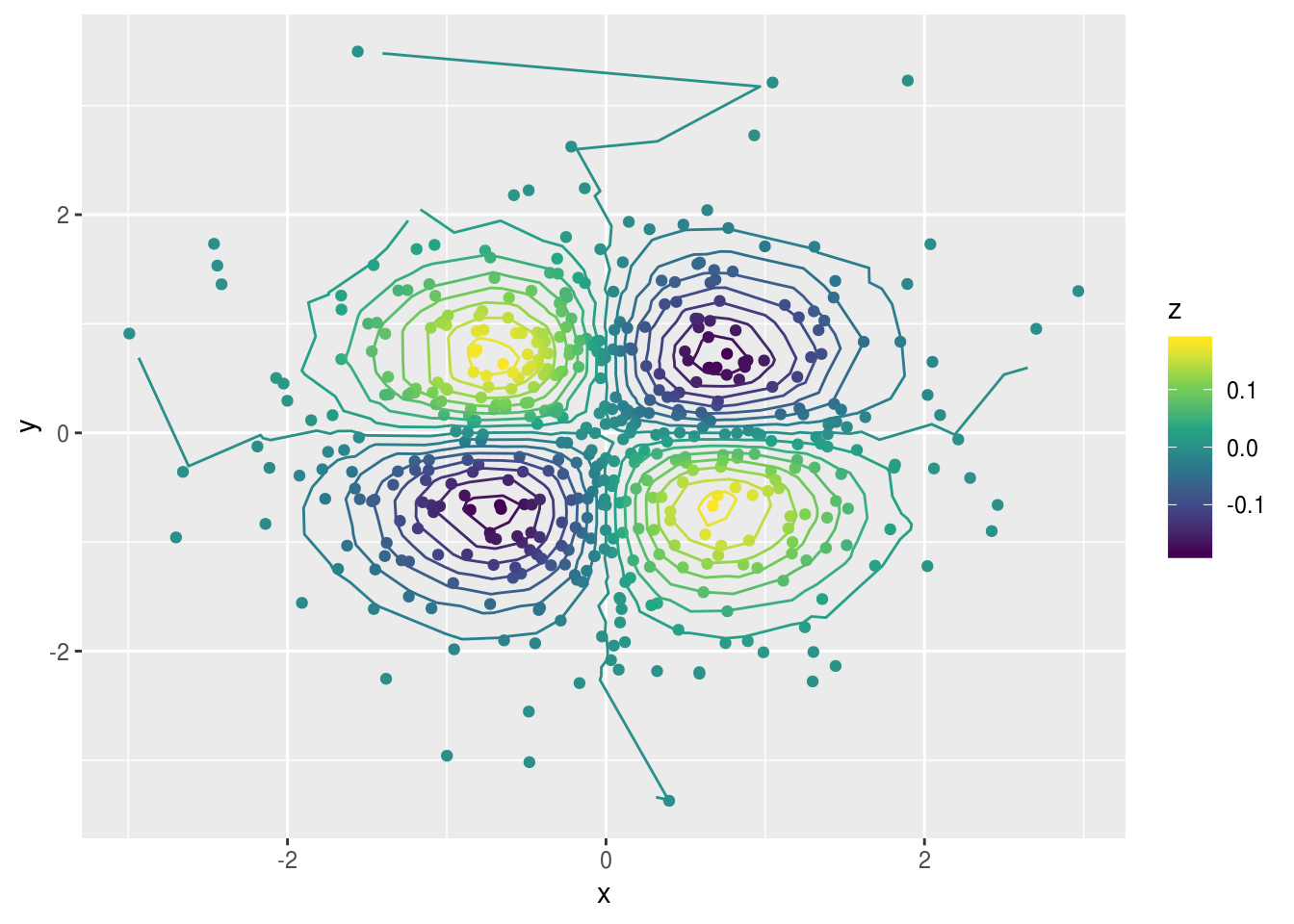
And voilà.
There’s always things to improve. For example, the possibility of using a custom function to compute parameters that depend on the data, but I believe that as it stands covers 80% of simple applications. I should also use a better name, but naming things is hard work.

